Classification Algorithms

Classification algorithms, handle linear and non-linear datasets a little differently. Classification algorithms have options that both resemble options available in clustering and linear regression algorithms. However, there are also options unique to Classification algorithms such as Naive Bayes and SVMs that utilize a Kernel trick to alter the dimensionality of a data set. The goal of a classification algorithms is to categorize something as "true" or "false."

The easiest way to imagine the shape of a classification algorithm is to think of a sine wave. The potential outputs are either 0 or 1, just like the origin and height of a normal sine wave. What differs between the algorithm methodology is largely how those values are obtained. Linear Classification is basically a sine function of normal linear regression. Decision Trees help break down the traits of cases where a label is true or false and address the presence or likely presence of those traits in a data point. Naive Bayes Classification is a fairly basic probability function to determine whether or not something is probable.

In fact, the Bayes classification function is defined as: the likelihood of an outcome multiplied by the probability of its priori, all divided by the marginal likelihood. For example, given a dataset of walkers and drivers, you would take the amount of walkers in a cluster of a data set, and divide them by the entire amount of points in the cluster. You would multiply that number by the size of the cluster you chose against the size of the entire data point. Then the denominator of the equation would be the number of walkers throughout the entire data set divided by the entire data set. You can see it in action below as I determine the likelihood of a circle being blue. Since the cluster I am working with matters it will be a little higher than the actual distribution of blue circles in the entire data set. This is because the goal is to determine the probability of a point fitting within a particular point of the data set, not in the data set altogether. There are other clusters I could have chosen where the probability would be 0 or less than 20%.

While all that is nice, sometimes data sets will be non-linear. In those cases a Support Vector Machine is necessary with a kernel function is necessary and the Radial Basis Function kernel is very popular in Machine Learning. An RBF kernel adds extra dimensionality to a data set in order to create a trend it can put onto a 2D plot. The image below sort of outlines that process. Also please note that no data set in this example is on the green plane. I should have drawn that better.

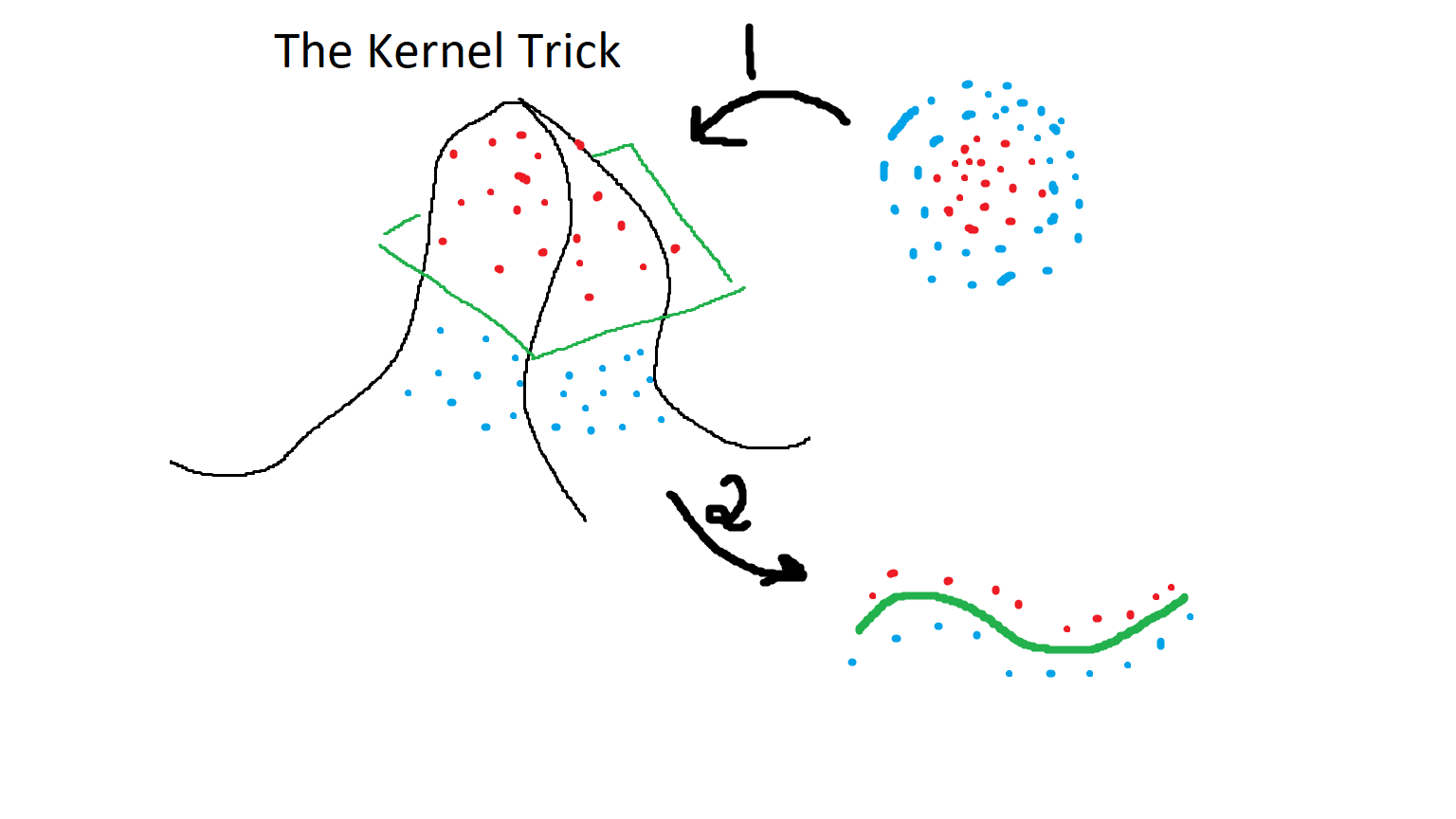
The image showed the kernel trick in action, which is basically plotting a 2D circle into three dimensions. The trend line is represented by a flat plane that would slice through all the possible values, and the data points that were in the circle would be plotted onto a 2D plane relative to its position with respect to the plane. For example, any point that sits on the plane will sit on the line in the final 2D result, otherwise the data point would sit above or below the line depending on its position relative to the plane. A plane in this case is a flat, one-sided 2D surface in a 3D space. It is worth noting that an RBF is not the only kernel available for non-linear data sets, and they can alter the outcome so choose wisely. The Confusion Matrix is a tool that can help us decide upon an algorithm most appropriate for a linear distribution, or the most appropriate kernel to use with SVM for non-linear data sets.

A typical confusion matrix is broken up into four parts: True Positives, False Positives, False Negatives, and True Negatives. There are two criteria that you should keep in mind when you use a confusion matrix. First, the obvious criteria is ensuring the true positive count is higher than the true negative count. That means that the algorithm is doing a good job determining where data points fit. Second, since no algorithm is perfect it is important to consider whether false positives (Type I errors) or false negatives (Type II errors) are safer given the circumstances. Falsely predicting someone is diabetic and running more tests is safer than falsely predicting they are not diabetic. Of course, this is all even assuming that the situation is appropriate for a classification algorithm.

All-in-all, classification algorithms are incredibly powerful algorithms that can help us determine the likelihood of a data point fitting within a cluster of data. It can also help us determine the likelihood of a single data point fitting within a distribution. Classification algorithms can be applied to both linear and non-linear data sets. However, they are not always appropriate to apply to a data set. Confusion matrices can help a scientist determine an algorithms accuracy, but it's also important to consider whether using a classification algorithm is even ethical. The real world can be a fluid place, and capturing the truth at a single very small point in time can be dangerous. As always, I have a GitHub repository full of classification algorithms.